What is reyna?
A lightweight Python package for solving partial differential equations (PDEs) using polygonal discontinuous Galerkin finite elements, providing a flexible and efficient way to approximate solutions to complex PDEs.
Features
Support for various polygonal element types (e.g., triangles, quadrilaterals, etc.)
Easy-to-use API for mesh generation, assembly, and solving PDEs.
High performance with optimized solvers for large-scale problems.
Supports linear advection-diffusion-reaction equations.
Extensible framework: easily integrate custom element types, solvers, or boundary conditions.
Installation
You can install the package via pip. First, clone the repository and then install it using pip:
Install from PyPI:
pip install reyna
Install from source:
pip install git+https://github.com/mattevs24/reyna.git
Please use a Python version 3.8-<3.12 to ensure that all features work as expected.
Example Usage
Create a Simple Mesh
A simple example to begin with is the RectangleDomain object. This requires just the bounding
box as an input. In this case, we consider the unit square; \([0, 1]^2\). We then use poly_mesher
to generate a bounded Voronoi mesh of the domain. This uses Lloyd’s algorithm, which can produce
edges that are machine precision in length. To avoid this for benchmarking and other critical
purposes, use the cleaned keyword, set to True.
import numpy as np

from reyna.polymesher.two_dimensional.domains import RectangleDomain
from reyna.polymesher.two_dimensional.main import poly_mesher

domain = RectangleDomain(bounding_box=np.array([[0, 1], [0, 1]]))
poly_mesh = poly_mesher(domain, max_iterations=10, n_points=1024)
Generating the Geometry Information
The DGFEM code requires additional information about the mesh to be able to run, including which edges
are boundary edges and their corresponding normals as well as information on a given subtriagulation to
be able to numerically integrate with the required precision. This is done using the DGFEMgeometry function.
from reyna.geometry.two_dimensional.DGFEM import DGFEMGeometry

geometry = DGFEMGeometry(poly_mesh)
Defining the Partial Differential Equation
To define the PDE, we need to call the DGFEM object. We then add data in the form of the general coefficients for a (up-to) second order PDE of the form
where \(a\) is the diffusion tensor, \(b\) is the advection vector, \(c\) is the reation functional and \(f\) is the forcing functional. All of these functions must be able to take in a (N, 2) array of points and output tensors of the correct shape; (N, 2, 2), (N, 2), (N,) and (N,) respectively. An example is given
def diffusion(x):
    out = np.zeros((x.shape[0], 2, 2), dtype=np.float64)
    for i in range(x.shape[0]):
        out[i, 0, 0] = 1.0
        out[i, 1, 1] = 1.0
    return out

advection = lambda x: np.ones(x.shape, dtype=float)
reaction = lambda x: np.pi ** 2 * np.ones(x.shape[0], dtype=float)
forcing = lambda x: np.pi * (np.cos(np.pi * x[:, 0]) * np.sin(np.pi * x[:, 1]) +
                             np.sin(np.pi * x[:, 0]) * np.cos(np.pi * x[:, 1])) + \
                    3.0 * np.pi ** 2 * np.sin(np.pi * x[:, 0]) * np.sin(np.pi * x[:, 1])

solution = lambda x: np.sin(np.pi * x[:, 0]) * np.sin(np.pi * x[:, 1])
We use the solution function here as the boundary conditions for the solver.
Adding data and Assembly
We can now call the solver, add the data and assemble.
from reyna.DGFEM.two_dimensional.main import DGFEM

dg = DGFEM(geometry, polynomial_degree=1)

dg.add_data(
    diffusion=diffusion,
    advection=advection,
    reaction=reaction,
    dirichlet_bcs=solution,
    forcing=forcing
    )

dg.dgfem(solve=True)
Setting the solve input to True generates the solution vector. If this is False, just the
stiffness matrix and data vector are generated.
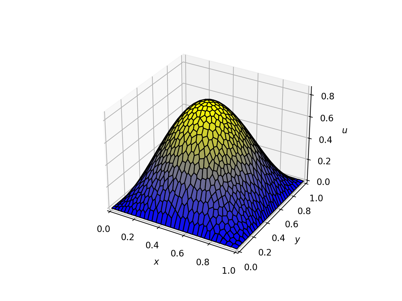
Visualize the solution
We also have a method to plot the data, plot_DG, but this is limited to polynomial degree 1
with limited support for polynomial degree 0. See the example below
dg.plot_DG()
or for more customisation, use the function plot_DG,
from reyna.DGFEM.two_dimensional.tools import plot_DG

plot_DG(dg.solution, geometry, dg.polydegree)
For the given example, we have the solution plot
Benchmarking
We have a benchmarking file that may be run availible in the main DGFEM directory. But we also provide an example of the code to be able to calculate yourself
def grad_solution(x: np.ndarray):
    u_x = np.pi * np.cos(np.pi * x[:, 0]) * np.sin(np.pi * x[:, 1])
    u_y = np.pi * np.sin(np.pi * x[:, 0]) * np.cos(np.pi * x[:, 1])

    return np.vstack((u_x, u_y)).T

dg_error, l2_error, h1_error = dg.errors(
    exact_solution=solution,
    div_advection=lambda x: np.zeros(x.shape[0]),
    grad_exact_solution=grad_solution
)
Often, the error rate is calcuated against the maximal cell diameter; the code for this is included in
the DGFEM class under the h method as well as the DGFEMgeometry class under the h method (DGFEMgeometry
additionally contains all the local values of h across the mesh).
h = dg.h
h = geometry.h
Note that in a purely advection/diffusion problem, some of the norms are unavailable and return
a None value.
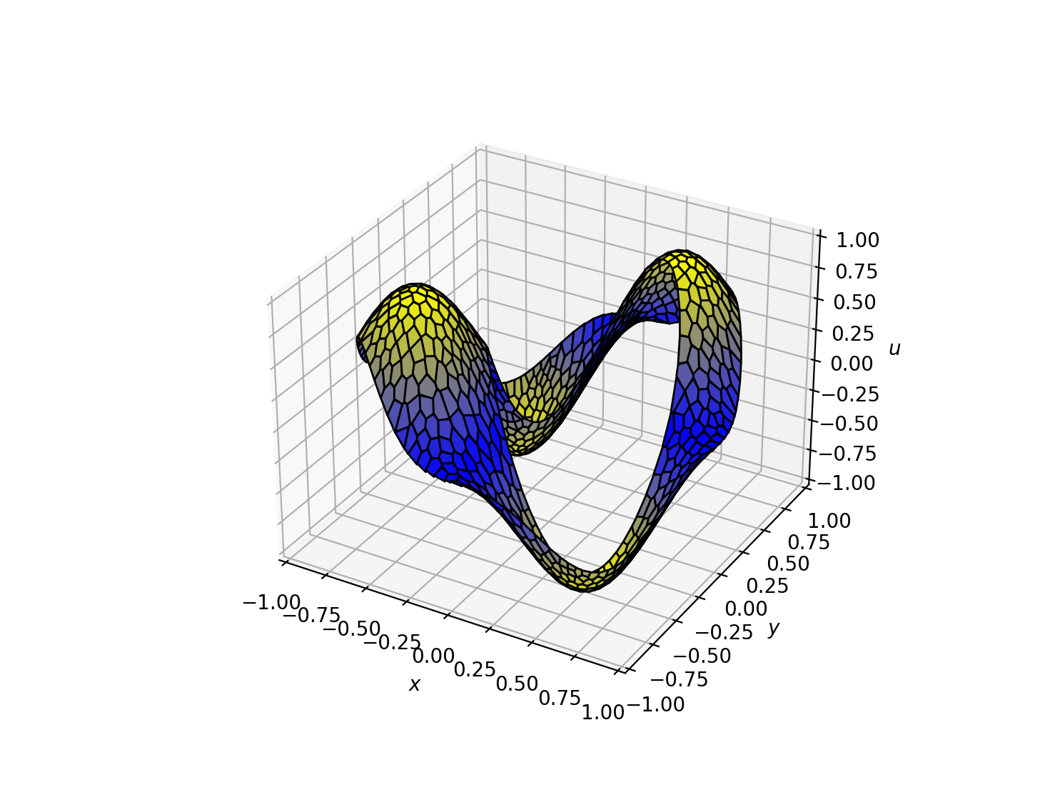
A more advanced Domain Example
There are many predefined domains in the reyna/polymesher/two_dimensional/domains folder including this
more advanced CircleCircleDomain() domain;
Example Notebooks
There are Jupyter notebooks availible in the GitHub repository which run through several examples of this package in action. This also runs through examples of benchmarking and custom domain generation.
Documentation
For detailed usage and API documentation, please visit our (soon to be) readthedocs. The above example and notebooks cover most cases and the current docstrings are very thorough.
Contributing
This project accepts contributions - see the CONTRIBUTING.md file for details.
License
This project is licensed under the MIT License - see the LICENSE.md file for details.
Credits & Acknowledgements
This package was developed by mattevs24 during a PhD programme funded by the French Alternative Energies and Atomic Energy Commission. A Special thanks to the support of Ansar Calloo, Fraçois Madiot throughout the PhD so far. A further thank you to my interal supervisors Tristan Pryer and Luca Zanetti for their role in this project too and useful feedback on usability and support. Finally, a thank you to Reyna who puts up with all this nonsense!
Upcoming Updates
There are many features that remain to add to this code! We hope to add support for the following features
Neumann and Robin boundary conditions: further support for more advanced boundary conditions that fit naturally into the DGFEM formulation.
Mixed boundary conditions: support for multiple types of boundary conditions on the same domain.
3D DGFEM: implement a full three dimensional version of the code able to support the same functionality.
Package Contents
Subpackages: